Wordcloud of COVID-19 research in Malaysia

Let’s see how much research has been done in term of COVID-19 in Malaysia. In this analysis, we are going to use Scopus database to access the relevant research or papers. In this analysis we are going to use 4 specific parts of the scientific paper:

1. Title
2. Abstract
3. Author’s keywords
4. Scopus’s keywords

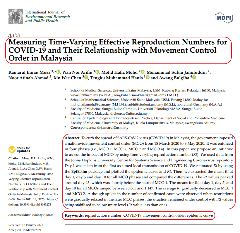Above is a sample of paper that shows the section of scientific paper that we are going to use in our analysis. The Scopus’s keywords are generated by the Scopus database, thus, it does not available on the paper.

So, the analysis will be applied separately on these 4 parts of the papers. Also, we are going to use map (equivalent to loop) since the flow of the analysis is similar.

Load the related packages. The main package is quanteda.

library(tidyverse)
library(quanteda)
library(quanteda.textstats)
library(quanteda.textplots)
library(patchwork)
library(wordcloud2)

I have uploaded the data that I downloaded from the Scopus database into my GitHub.

# Read data from GitHub repo
df <- read.csv("https://raw.githubusercontent.com/tengku-hanis/scopus-data/main/covid-malaysia.csv") %>% 
  janitor::clean_names() %>% 
  rename(title =i_title)

First, we need to tokenize the sentence. In other words, we break down the sentences into words.

# Tokenize
tok_list <- 
  df %>% 
  select(title, abstract, author_keywords, index_keywords) %>% 
  map(tokens, 
      remove_punct = T, 
      remove_numbers = T,               
      remove_symbols = T)

Next, we remove words that are not meaningful such ‘a’, ‘the’, etc. These words are known as stop words.

# Remove stop words
nostop_toks <- 
  tok_list %>% 
  map(tokens_select, 
      c(tidytext::stop_words$word, stopwords("en")), 
      selection = "remove")

Then, we create a document feature matrix (DFM). Basically DFM is a matrix that represent the frequency of each word (feature) in each document (in our case, paper or manuscript). Another name for DFM is document term matrix (DTM). quanteda uses the term DFM, some other packages use the term DTM.

Additionally, we also apply term frequency-inverse document frequency (TF-IDF) metrics. In scientific papers, the words such as ‘determine’, ‘conclusion’, ‘introduction’, etc are very frequent, and these words are not meaningful as well. Instead of removing manually one by one, we use TF-IDF. So, TF-IDF basically remove the words that are too common, thus we get only the relevant or important words.

# Create DFM and apply tf_idf
covid_dfm_list <- 
  nostop_toks %>% 
  map(dfm) %>% 
  map(dfm_tfidf)

# Plot top features
A <- 
  covid_dfm_list$title %>% 
  textstat_frequency(n = 15, force = T) %>% 
  ggplot(aes(x = reorder(feature, frequency), y = frequency)) +
  geom_point(size = 4, colour = "blueviolet") +
  coord_flip() +
  labs(x = NULL, y = "Frequency (tf-idf)") +
  theme_minimal() +
  labs(title = "Top relevant terms for covid research based on the title")

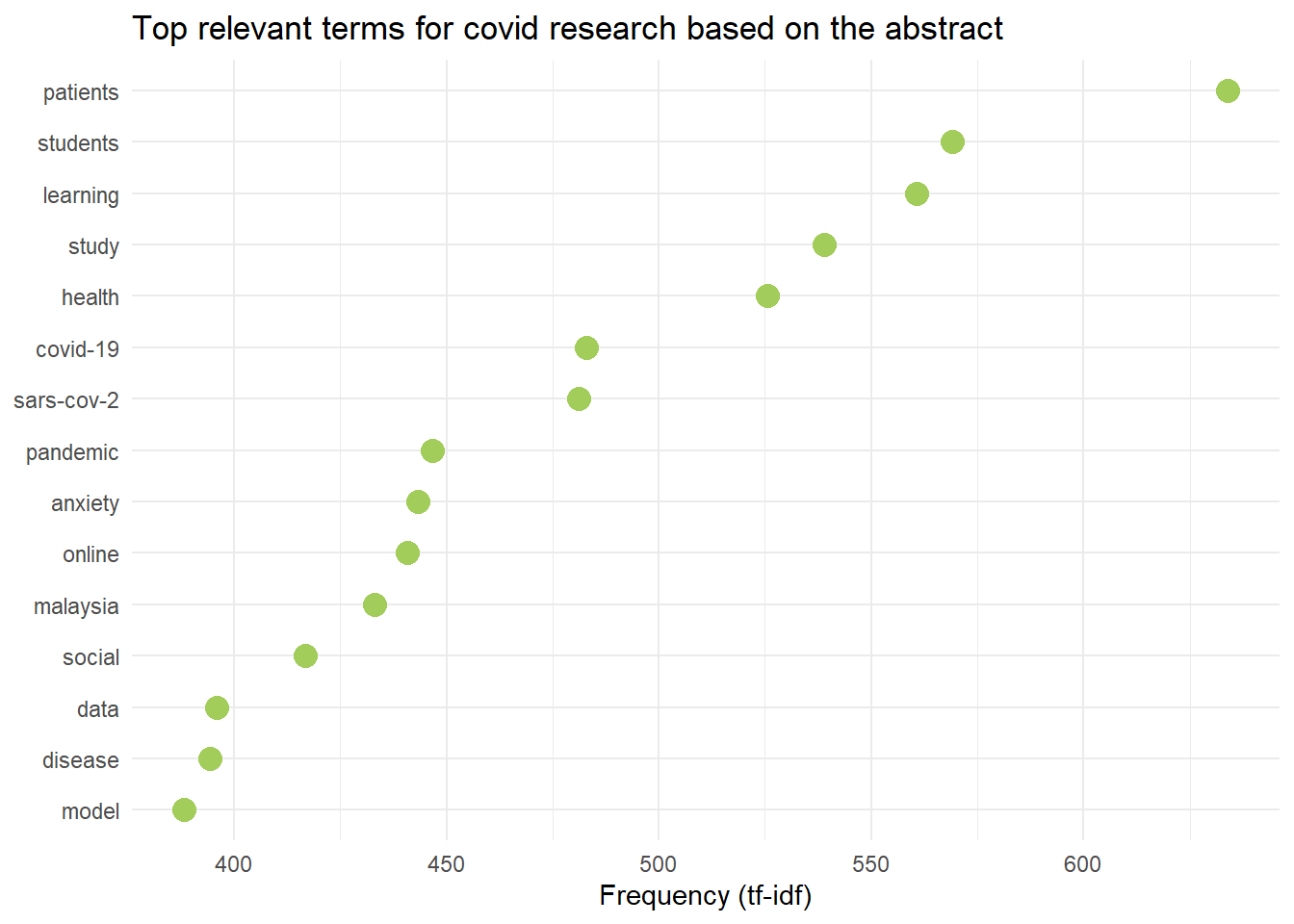
B <- 
  covid_dfm_list$abstract %>% 
  textstat_frequency(n = 15, force = T) %>% 
  ggplot(aes(x = reorder(feature, frequency), y = frequency)) +
  geom_point(size = 4, colour = "darkolivegreen3") +
  coord_flip() +
  labs(x = NULL, y = "Frequency (tf-idf)") +
  theme_minimal() +
  labs(title = "Top relevant terms for covid research based on the abstract")

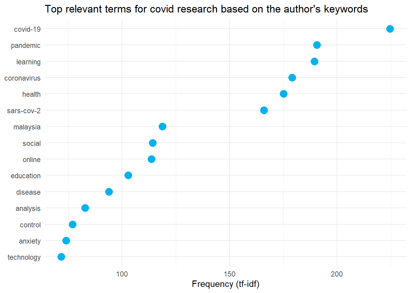
C <- 
  covid_dfm_list$author_keywords %>% 
  textstat_frequency(n = 15, force = T) %>% 
  ggplot(aes(x = reorder(feature, frequency), y = frequency)) +
  geom_point(size = 4, colour = "deepskyblue2") +
  coord_flip() +
  labs(x = NULL, y = "Frequency (tf-idf)") +
  theme_minimal() +
  labs(title = "Top relevant terms for covid research based on the author's keywords")

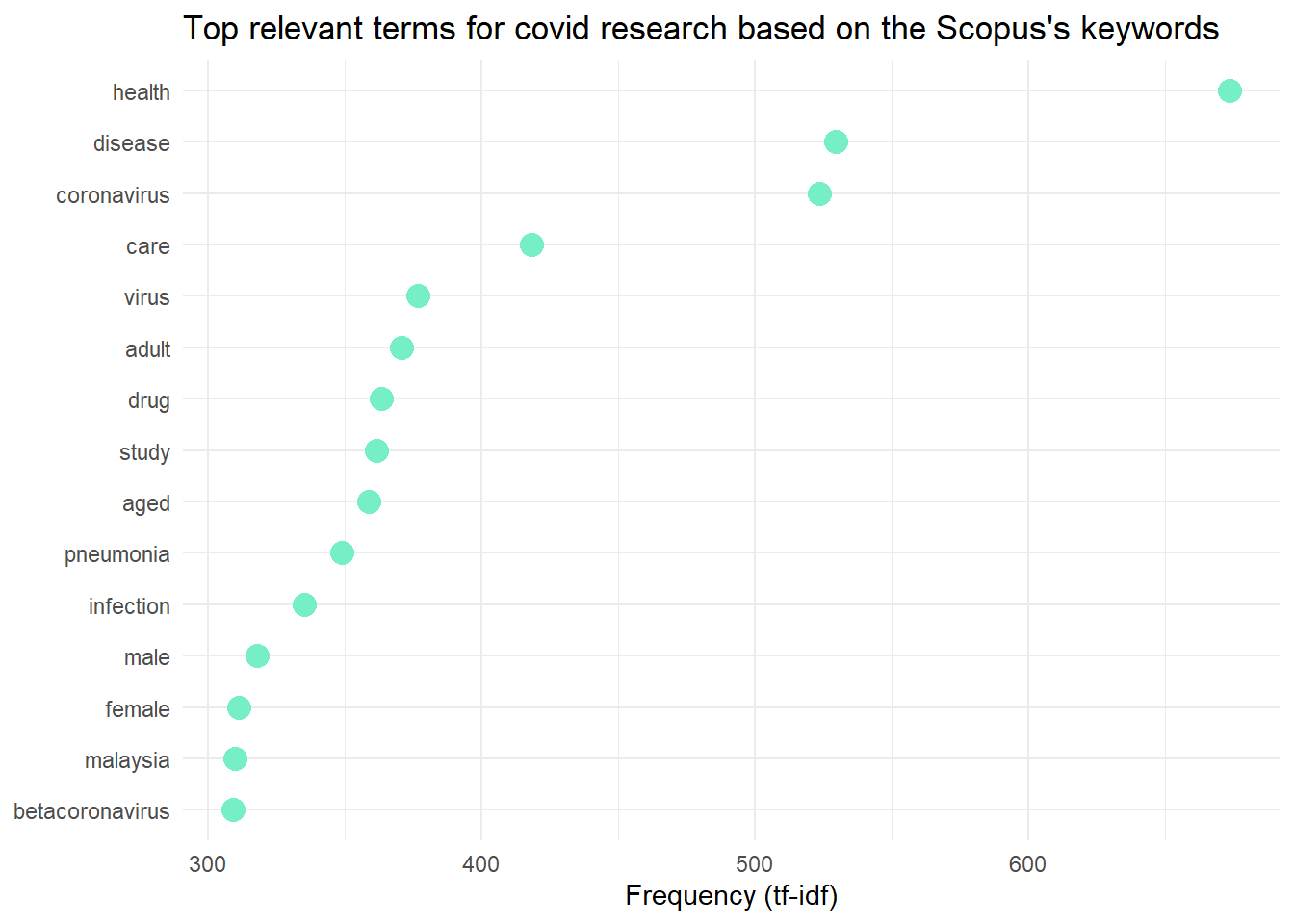
D <- 
  covid_dfm_list$index_keywords %>% 
  textstat_frequency(n = 15, force = T) %>% 
  ggplot(aes(x = reorder(feature, frequency), y = frequency)) +
  geom_point(size = 4, colour = "aquamarine2") +
  coord_flip() +
  labs(x = NULL, y = "Frequency (tf-idf)") +
  theme_minimal() +
  labs(title = "Top relevant terms for covid research based on the Scopus's keywords")

These are the plots of the most relevant terms in COVID-19 research in Malaysia.

covid_wc <- 
  covid_dfm_list %>% 
  map(textstat_frequency, force = T)

wordcloud2(covid_wc$title%>% 
             slice(1:1000) %>% 
             mutate(frequency = round(frequency)))

wordcloud2(covid_wc$abstract %>% 
             slice(1:1000) %>% 
             mutate(frequency = round(frequency)))

wordcloud2(covid_wc$author_keywords%>% 
             slice(1:1000) %>% 
             mutate(frequency = round(frequency)))

wordcloud2(covid_wc$index_keywords%>% 
             slice(1:1000) %>% 
             mutate(frequency = round(frequency)))