Mapping the states in Malaysia
I have written two blog posts about making map in R:
This post is sort of a continuation to the first blog post. I have shown how to plot a coordinate to a map in that post specifically for Malaysia.
However, using the two approaches in the previous blog post, we cannot plot the coordinate to a certain states in Malaysia. At least I am not unable to find how to do that after googling around. But, we can plot the borneo or peninsular of Malaysia using the two approaches.
Plot the peninsular of Malaysia (not the best way)
Load the necessary packages.
library(rworldmap)
library(tidyverse)
First, we get the data. The data is about desa clinic (klinik desa) in Malaysia.
clinicDesa <- read.csv("https://raw.githubusercontent.com/tengku-hanis/clinic-data/main/clinicdesa.csv")
head(clinicDesa)
## id facilities_id name address postcode
## 1 1 KD01010019 KLINIK DESA ASSAM BUBOK Jalan Batu Pahat 86400
## 2 2 KD01010020 KLINIK DESA BATU PUTIH Jalan Behor Temak 83000
## 3 3 KD01010021 KLINIK DESA BEROLEH Jalan Parit Besar 83300
## 4 4 KD01010022 KLINIK DESA BINDU Jalan Tongkang Pecah 83010
## 5 5 KD01010023 KLINIK DESA KAMPUNG BARU Jalan Parit Kemang 83710
## 6 6 KD01010024 KLINIK DESA KANGKAR BARU Jalan Meng Seng 85400
## city district state tel fax website email image latitude
## 1 Ayer Hitam Batu Pahat Johor NA NA NA NA 1.933330
## 2 Bagan Batu Pahat Johor NA NA NA NA 1.889100
## 3 Sri Gading Batu Pahat Johor NA NA NA NA 1.877890
## 4 Tongkang Pecah Batu Pahat Johor NA NA NA NA 1.901515
## 5 Parit Yaani Batu Pahat Johor NA NA NA NA 1.905120
## 6 Yong Peng Batu Pahat Johor NA NA NA NA 2.065310
## longitude likes rating status
## 1 103.1167 0 0 NEW
## 2 102.8778 0 0 NEW
## 3 102.9858 0 0 NEW
## 4 102.9665 0 0 NEW
## 5 103.0372 0 0 NEW
## 6 103.1248 0 0 NEWFirst we plot the data.
ggplot(clinicDesa, aes(longitude, latitude)) +
  geom_point() +
  theme_minimal()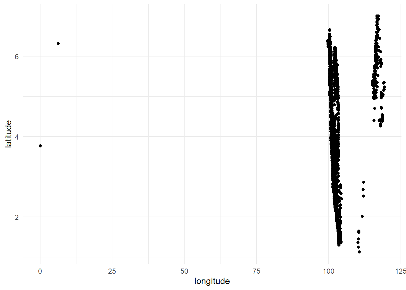
Remove the two points.
clinicDesa2 <- clinicDesa %>% filter(longitude > 25)Again, plot the updated data.
ggplot(clinicDesa2, aes(longitude, latitude)) +
  geom_point() +
  theme_minimal()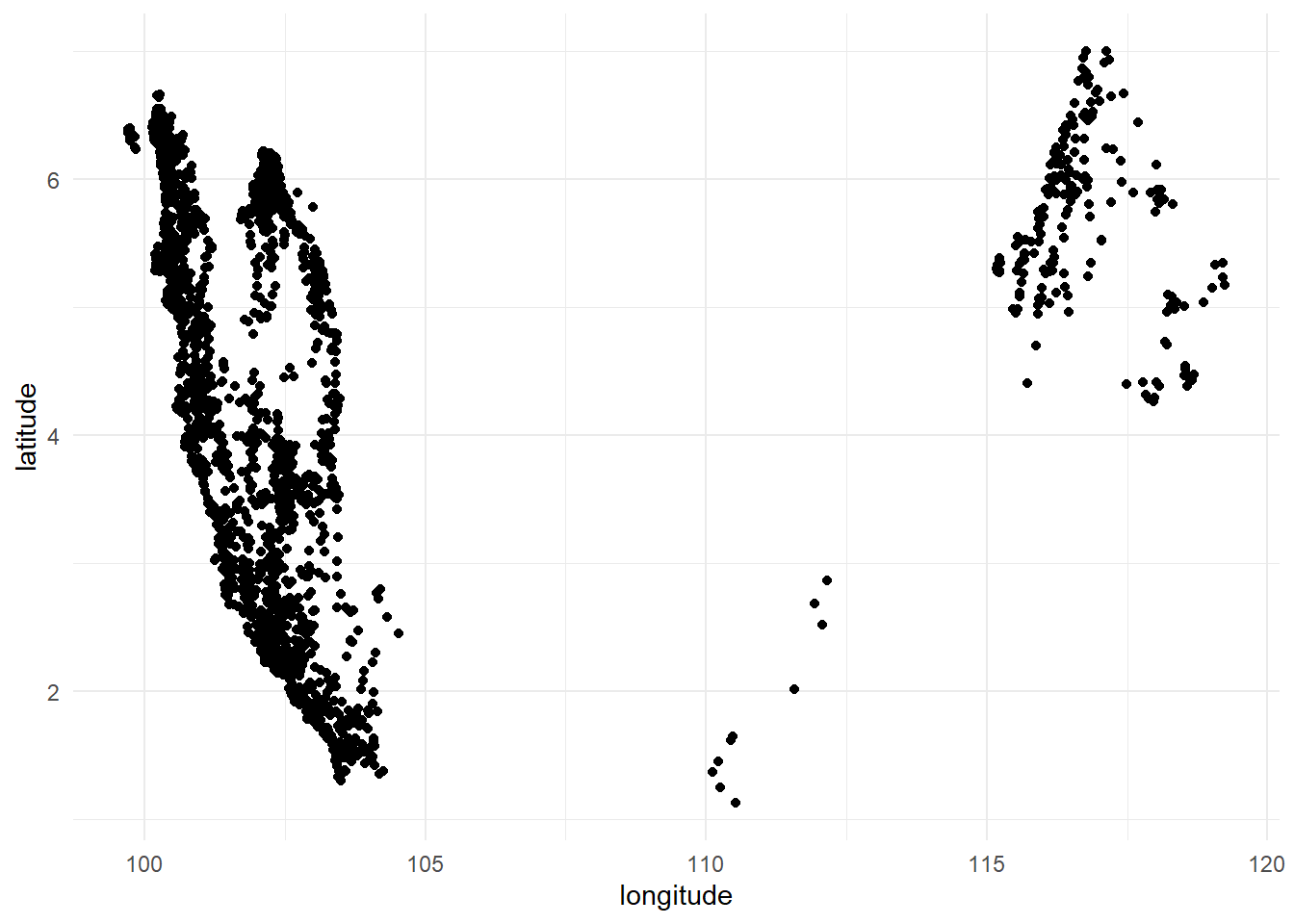
From the plot, we already know the left side consists of the coordinates in the peninsular of Malaysia. So, we can limit our plot by limit the longitude < 105 and longitude > 97.
# Get base map
global <- map_data("world")

# Plot
ggplot() +
  geom_polygon(data = global %>% filter(region == "Malaysia"), aes(x=long, y = lat, group = group),
               fill = "gray85") +
  coord_fixed(1.3) +
  geom_point(data = clinicDesa2, aes(x = longitude, y = latitude)) +
  theme_minimal() +
  xlab("Longitude") +
  ylab("Latitude") +
  labs(title = "Desa clinic in the peninsular of Malaysia",
       subtitle = "(Data last updated: Klinik Desa - 9 Mac 2021)",
       caption = expression(paste(italic("Sumber data: https://www.data.gov.my/data/ms_MY/group/pemetaan")))) +
  xlim(97, 105) #limit overall map to peninsular of Malaysia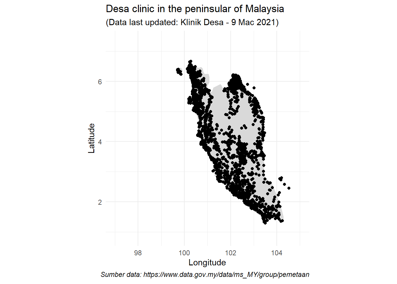
I am not going to re-explain the above and below codes as I have explain it in the previous blog post.
This approach also works with rworldmap.
# Get base map
world <- getMap(resolution = "low")
msia <- world[world@data$ADMIN == "Malaysia", ]

# Plot
ggplot() +
  geom_polygon(data = msia, aes(x = long, y = lat, group = group), fill = NA, colour = "black") +
  geom_point(data = clinicDesa2, aes(x = longitude, y = latitude)) +
  coord_quickmap() +
  theme_minimal() +
  xlab("Longitude") +
  ylab("Latitude") +
  labs(title = "Desa clinic in the peninsular of Malaysia",
       subtitle = "(Data last updated: Klinik Desa - 9 Mac 2021)",
       caption = expression(paste(italic("Sumber data: https://www.data.gov.my/data/ms_MY/group/pemetaan")))) +
  xlim(97, 105) #limit overall map to peninsular of Malaysia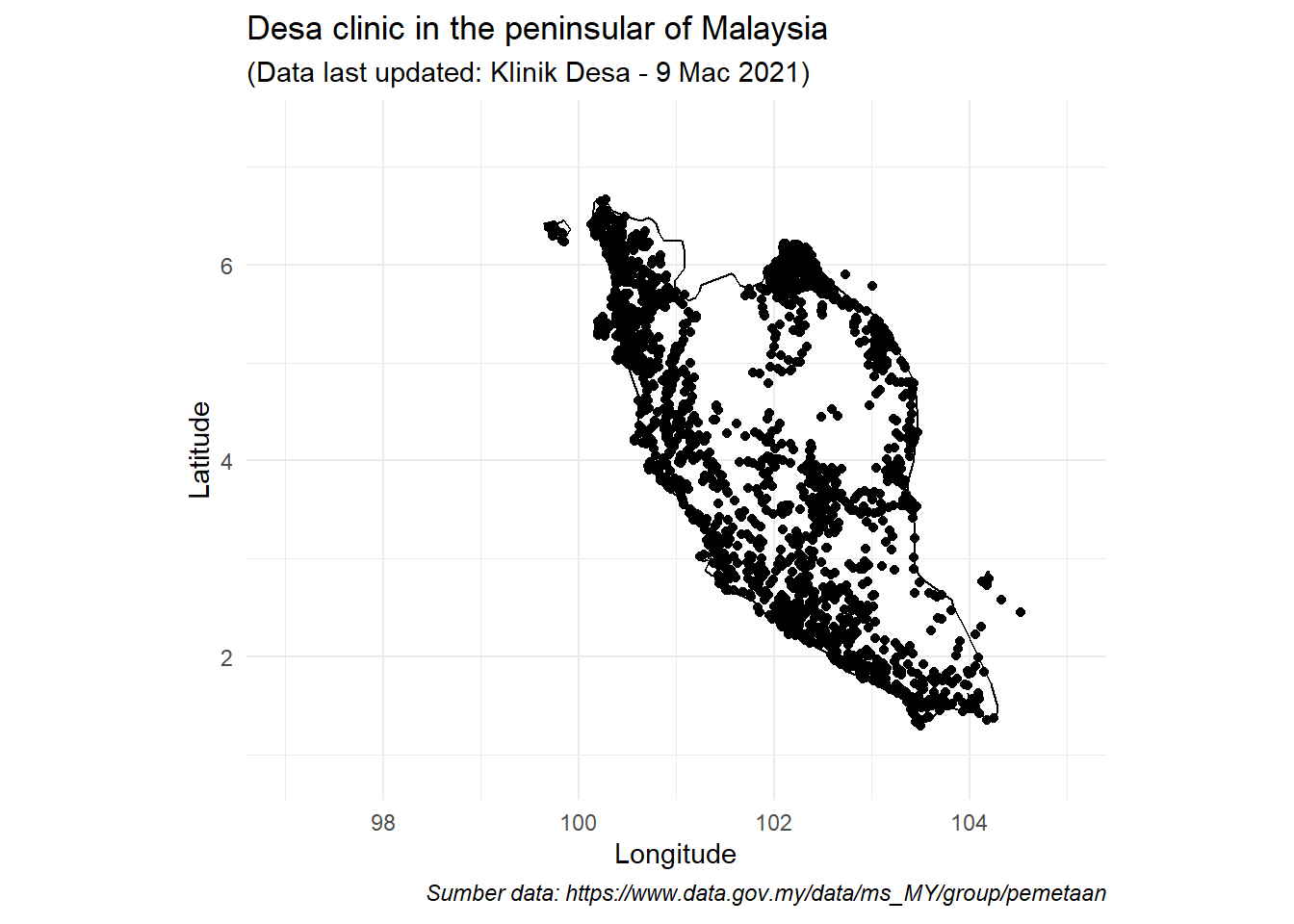
As we can see using the two approaches, we can plot the borne and peninsular sides of Malaysia. But, at least to my knowledge we cannot apply this approach if we want to plot a coordinate to certain states in Malaysia.
Plot the states in Malaysia
Load the necessary package.
library(geodata)
library(tidyterra)
As we can see from the package, we going to use a geodata package. tidyterra is used to supplements the ggplot. First, let’s limit the data into desa clinics in Terengganu only.
clinic_trg <-
  clinicDesa %>%
  filter(state == "Terengganu") %>%
  dplyr::select(latitude, longitude)
head(clinic_trg)
## latitude longitude
## 1 5.48533 102.4914
## 2 5.81578 102.5778
## 3 5.70886 102.4892
## 4 5.75722 102.5303
## 5 5.67444 102.6289
## 6 5.69875 102.5430Now we get the map from the geodata package with the boundaries at the district level.
Malaysia <- gadm(country = "MYS", level = 2, path=tempdir())We can use the below information to limit the map to Terengganu state only.
Malaysia$NAME_1## [1] "Johor" "Johor" "Johor" "Johor"
## [5] "Johor" "Johor" "Johor" "Johor"
## [9] "Johor" "Johor" "Kedah" "Kedah"
## [13] "Kedah" "Kedah" "Kedah" "Kedah"
## [17] "Kedah" "Kedah" "Kedah" "Kedah"
## [21] "Kedah" "Kedah" "Kelantan" "Kelantan"
## [25] "Kelantan" "Kelantan" "Kelantan" "Kelantan"
## [29] "Kelantan" "Kelantan" "Kelantan" "Kelantan"
## [33] "Kuala Lumpur" "Labuan" "Melaka" "Melaka"
## [37] "Melaka" "Negeri Sembilan" "Negeri Sembilan" "Negeri Sembilan"
## [41] "Negeri Sembilan" "Negeri Sembilan" "Negeri Sembilan" "Negeri Sembilan"
## [45] "Pahang" "Pahang" "Pahang" "Pahang"
## [49] "Pahang" "Pahang" "Pahang" "Pahang"
## [53] "Pahang" "Pahang" "Pahang" "Perak"
## [57] "Perak" "Perak" "Perak" "Perak"
## [61] "Perak" "Perak" "Perak" "Perak"
## [65] "Perak" "Perlis" "Pulau Pinang" "Pulau Pinang"
## [69] "Pulau Pinang" "Pulau Pinang" "Pulau Pinang" "Putrajaya"
## [73] "Sabah" "Sabah" "Sabah" "Sabah"
## [77] "Sabah" "Sabah" "Sabah" "Sabah"
## [81] "Sabah" "Sabah" "Sabah" "Sabah"
## [85] "Sabah" "Sabah" "Sabah" "Sabah"
## [89] "Sabah" "Sabah" "Sabah" "Sabah"
## [93] "Sabah" "Sabah" "Sabah" "Sabah"
## [97] "Sabah" "Sarawak" "Sarawak" "Sarawak"
## [101] "Sarawak" "Sarawak" "Sarawak" "Sarawak"
## [105] "Sarawak" "Sarawak" "Sarawak" "Sarawak"
## [109] "Sarawak" "Sarawak" "Sarawak" "Sarawak"
## [113] "Sarawak" "Sarawak" "Sarawak" "Sarawak"
## [117] "Sarawak" "Sarawak" "Sarawak" "Sarawak"
## [121] "Sarawak" "Sarawak" "Sarawak" "Sarawak"
## [125] "Sarawak" "Sarawak" "Sarawak" "Sarawak"
## [129] "Selangor" "Selangor" "Selangor" "Selangor"
## [133] "Selangor" "Selangor" "Selangor" "Selangor"
## [137] "Selangor" "Trengganu" "Trengganu" "Trengganu"
## [141] "Trengganu" "Trengganu" "Trengganu" "Trengganu"So, this is the plot for Terengganu.
Trg <- Malaysia[138:144,]
plot(Trg)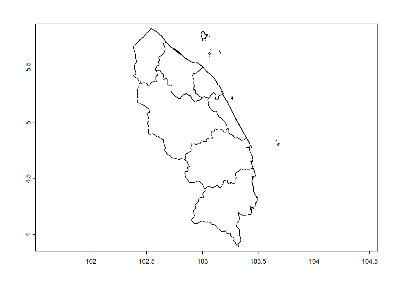
We going to the map this in ggplot, and stacked the map layer with the coordinate layer.
ggplot() +
  geom_spatvector(data = Trg, color = "grey", fill = NA) +
  geom_point(data = clinic_trg, aes(x = longitude, y = latitude, color = "red")) +
  theme_minimal() +
  theme(legend.position = "none") +
  xlab("Longitude") +
  ylab("Latitude") +
  labs(title = "Desa clinic in Terengganu, Malaysia",
       subtitle = "(Data last updated: Klinik Desa - 9 Mac 2021)",
caption = expression(paste(italic("Sumber data: https://www.data.gov.my/data/ms_MY/group/pemetaan")))) 
geom_spatvector is from tidyterra package. Alternatively, we can plot using geom_sfbut we need to convert the SpatVector data into sf object using sf::st_as_sf.
ggplot(data = sf::st_as_sf(Trg)) +
  geom_sf(color = "grey", fill = NA) +
  geom_point(data = clinic_trg, aes(x = longitude, y = latitude, color = "red")) +
  theme_minimal() +
  theme(legend.position = "none") +
  xlab("Longitude") +
  ylab("Latitude") +
  labs(title = "Desa clinic in Terengganu, Malaysia",
       subtitle = "(Data last updated: Klinik Desa - 9 Mac 2021)",
caption = expression(paste(italic("Sumber data: https://www.data.gov.my/data/ms_MY/group/pemetaan")))) 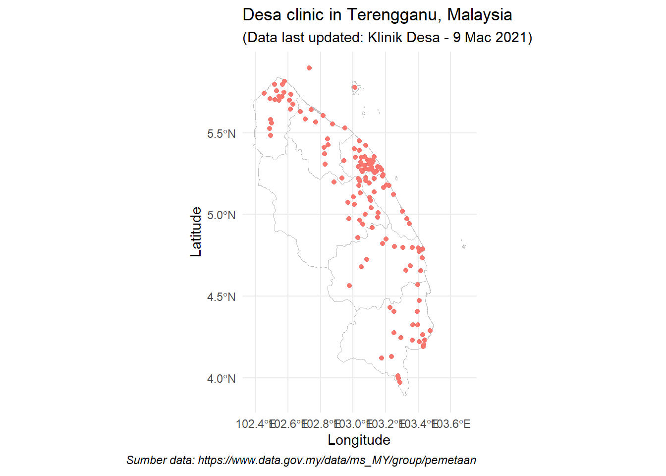
Both approaches produce the same plot.
We can further add district labels to the plots. For example, using the geom_sf, we can stack it with geom_sf_label layer. We can alternatively use theme_void to remove the background and the map axis.
ggplot(data = sf::st_as_sf(Trg)) +
  geom_sf(color = "grey", fill = NA) +
  geom_sf_label(aes(label = NAME_2)) +
  geom_point(data = clinic_trg, aes(x = longitude, y = latitude, color = "red")) +
  theme_void() +
  theme(legend.position = "none") +
  xlab("Longitude") +
  ylab("Latitude") +
  labs(title = "Desa clinic in Terengganu, Malaysia",
       subtitle = "(Data last updated: Klinik Desa - 9 Mac 2021)",
caption = expression(paste(italic("Sumber data: https://www.data.gov.my/data/ms_MY/group/pemetaan")))) 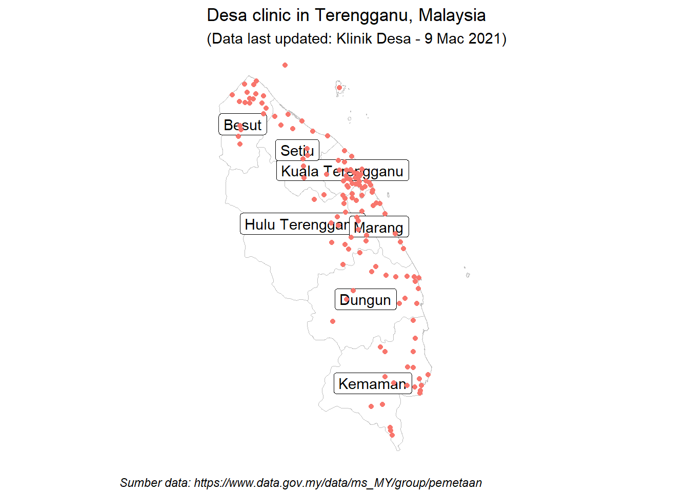
Tengku Muhammad Hanis
Lead academic trainer
My research interests include medical statistics and machine learning application.