Using UMAP preprocessing for image classification

UMAP

Uniform manifold approximation and projection or in short UMAP is a type of dimension reduction techniques. So, basically UMAP will project a set of features into a smaller space. UMAP can be a supervised technique in which we give a label or an outcome or an unsupervised one. For those interested to know in detail how UMAP works can refer to this reference. For those prefer a much simpler or shorter version of it, I recommend a YouTube video by Joshua Starmer.

Example in R

We going to see how to apply a UMAP techniques for image preprocessing and further classify the images using kNN and naive bayes.

These are the packages that we need.

library(keras) #for data and reshape to tabular format
library(tidymodels)
library(embed) #for umap
library(discrim) #for naive bayes model

We going to use the famous MNIST dataset. This dataset contained a handwritten digit from 0 to 9. This dataset is available in keras package.

mnist_data <- dataset_mnist()

## Loaded Tensorflow version 2.2.0

image_data <- mnist_data$train$x
image_labels <- mnist_data$train$y
image_data %>% dim()

## [1] 60000    28    28

For example this is the image for the second row.

image_data[2, 1:28, 1:28] %>% 
  t() %>% 
  image(col = gray.colors(256))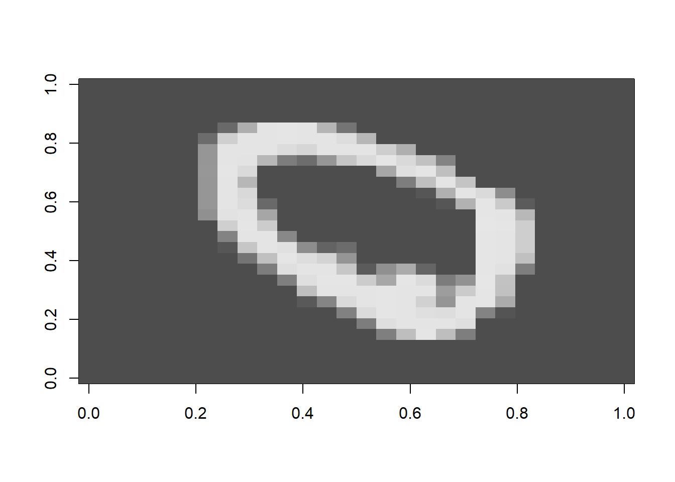

Next, we going to change the image into a tabular data frame format. We going to limit the data to the first 1000 rows or images out of the total 6000 images.

# Reformat to tabular format
image_data <- array_reshape(image_data, dim = c(60000, 28*28))
image_data %>% dim()

## [1] 60000   784

image_data <- image_data[1:10000,]
image_labels <- image_labels[1:10000]

# Reformat to data frame
full_data <- 
  data.frame(image_data) %>% 
  bind_cols(label = image_labels) %>% 
  mutate(label = as.factor(label))

Then, we going to split the data and create a 3-folds cross-validation sets for the sake of simplicity.

# Split data
set.seed(123)
ind <- initial_split(full_data)
data_train <- training(ind)  
data_test <- testing(ind)

# 10-folds CV
set.seed(123)
data_cv <- vfold_cv(data_train, v = 3)

For recipe specification, we going to scale and center all the predictor after creating a new variable using step_umap(). Notice that in step_umap() we supply the outcome and we tune the number of components (num_comp).

rec <- 
  recipe(label ~ ., data = data_train) %>% 
  step_umap(all_predictors(), outcome = vars(label), num_comp = tune()) %>% 
  step_center(all_predictors()) %>% 
  step_scale(all_predictors())

We create a a base workflow.

wf <- 
  workflow() %>% 
  add_recipe(rec) 

We going to use two models as classifier:

1. kNN
   
2. Naive bayes

For each classifier, we going to create a regular grid of parameters to be tuned and further run a regular grid search.

For kNN.

# knn model
knn_mod <- 
  nearest_neighbor(neighbors = tune()) %>% 
  set_mode("classification") %>% 
  set_engine("kknn")

# knn grid
knn_grid <- grid_regular(neighbors(), num_comp(range = c(2, 8)), levels = 3)

# Tune grid search
knn_tune <- 
  tune_grid(
  wf %>% add_model(knn_mod),
  resamples = data_cv,
  grid = knn_grid, 
  control = control_grid(verbose = F)
)

For naive bayes.

# nb model
nb_mod <- 
  naive_Bayes(smoothness = tune()) %>% 
  set_mode("classification") %>% 
  set_engine("naivebayes")

# nb grid
nb_grid <- grid_regular(smoothness(), num_comp(range = c(2, 10)), levels = 3)

# Tune grid search
nb_tune <- 
  tune_grid(
    wf %>% add_model(nb_mod),
    resamples = data_cv,
    grid = nb_grid, 
    control = control_grid(verbose = F)
  )

Let’s see our tuning performance of our model.

# knn model
knn_tune %>% 
  show_best("roc_auc")

## # A tibble: 5 x 8
##   neighbors num_comp .metric .estimator  mean     n  std_err .config            
##       <int>    <int> <chr>   <chr>      <dbl> <int>    <dbl> <chr>              
## 1        10        8 roc_auc hand_till  0.961     3 0.000268 Preprocessor3_Mode~
## 2        10        5 roc_auc hand_till  0.961     3 0.000421 Preprocessor2_Mode~
## 3         5        8 roc_auc hand_till  0.959     3 0.000757 Preprocessor3_Mode~
## 4        10        2 roc_auc hand_till  0.959     3 0.000737 Preprocessor1_Mode~
## 5         5        5 roc_auc hand_till  0.958     3 0.000740 Preprocessor2_Mode~

knn_tune %>% 
  show_best("accuracy")

## # A tibble: 5 x 8
##   neighbors num_comp .metric  .estimator  mean     n std_err .config            
##       <int>    <int> <chr>    <chr>      <dbl> <int>   <dbl> <chr>              
## 1        10        8 accuracy multiclass 0.914     3 0.00104 Preprocessor3_Mode~
## 2         5        8 accuracy multiclass 0.913     3 0.00315 Preprocessor3_Mode~
## 3        10        5 accuracy multiclass 0.912     3 0.00114 Preprocessor2_Mode~
## 4         5        5 accuracy multiclass 0.91      3 0.00139 Preprocessor2_Mode~
## 5        10        2 accuracy multiclass 0.910     3 0.00175 Preprocessor1_Mode~

# nb model
nb_tune %>% 
  show_best("roc_auc")

## # A tibble: 5 x 8
##   smoothness num_comp .metric .estimator  mean     n  std_err .config           
##        <dbl>    <int> <chr>   <chr>      <dbl> <int>    <dbl> <chr>             
## 1        1.5       10 roc_auc hand_till  0.971     3 0.000400 Preprocessor3_Mod~
## 2        1.5        6 roc_auc hand_till  0.971     3 0.000997 Preprocessor2_Mod~
## 3        1         10 roc_auc hand_till  0.971     3 0.000634 Preprocessor3_Mod~
## 4        1          6 roc_auc hand_till  0.970     3 0.00124  Preprocessor2_Mod~
## 5        0.5       10 roc_auc hand_till  0.969     3 0.000808 Preprocessor3_Mod~

nb_tune %>% 
  show_best("accuracy")

## # A tibble: 5 x 8
##   smoothness num_comp .metric  .estimator  mean     n  std_err .config          
##        <dbl>    <int> <chr>    <chr>      <dbl> <int>    <dbl> <chr>            
## 1        1         10 accuracy multiclass 0.913     3 0.000481 Preprocessor3_Mo~
## 2        1.5       10 accuracy multiclass 0.913     3 0.000267 Preprocessor3_Mo~
## 3        0.5       10 accuracy multiclass 0.912     3 0.000462 Preprocessor3_Mo~
## 4        1.5        6 accuracy multiclass 0.911     3 0.00135  Preprocessor2_Mo~
## 5        1          6 accuracy multiclass 0.910     3 0.00157  Preprocessor2_Mo~

Next, we going to select the best model from the tuned parameters and finalise our model using last_fit().

For knn model.

# Finalize
knn_best <- knn_tune %>% select_best("roc_auc")
knn_rec <- 
  recipe(label ~ ., data = data_train) %>% 
  step_umap(all_predictors(), outcome = vars(label), num_comp = knn_best$num_comp) %>% 
  step_center(all_predictors()) %>% 
  step_scale(all_predictors())

knn_wf <- 
  workflow() %>% 
  add_recipe(knn_rec) %>% 
  add_model(knn_mod) %>% 
  finalize_workflow(knn_best) 

# Last fit
knn_lastfit <- 
  knn_wf %>% 
  last_fit(ind)

For naive bayes model.

# Finalize
nb_best <- nb_tune %>% select_best("roc_auc")
nb_rec <- 
  recipe(label ~ ., data = data_train) %>% 
  step_umap(all_predictors(), outcome = vars(label), num_comp = nb_best$num_comp) %>% 
  step_center(all_predictors()) %>% 
  step_scale(all_predictors())

nb_wf <- 
  workflow() %>% 
  add_recipe(nb_rec) %>% 
  add_model(nb_mod) %>% 
  finalize_workflow(nb_best) 

# Last fit
nb_lastfit <- 
  nb_wf %>% 
  last_fit(ind)

Let’s see the model performance on the testing data.

knn_lastfit %>% 
  collect_metrics() %>% 
  mutate(model = "knn") %>% 
  dplyr::bind_rows(nb_lastfit %>% 
                     collect_metrics() %>% 
                     mutate(model = "nb")) %>% 
  select(-.config)

## # A tibble: 4 x 4
##   .metric  .estimator .estimate model
##   <chr>    <chr>          <dbl> <chr>
## 1 accuracy multiclass     0.938 knn  
## 2 roc_auc  hand_till      0.971 knn  
## 3 accuracy multiclass     0.936 nb   
## 4 roc_auc  hand_till      0.980 nb

These are the confusion matrices.

knn_lastfit %>% 
  collect_predictions() %>%
  conf_mat(label, .pred_class) %>% 
  autoplot(type = "heatmap") +
  labs(title = "Confusion matrix - kNN")

nb_lastfit %>% 
  collect_predictions() %>%
  conf_mat(label, .pred_class) %>% 
  autoplot(type = "heatmap") +
  labs(title = "Confusion matrix - naive bayes")

Lastly, we can compare the ROC plots for each class.

knn_lastfit %>% 
  collect_predictions() %>%
  mutate(id = "knn") %>% 
  bind_rows(
    nb_lastfit %>% 
      collect_predictions() %>% 
      mutate(id = "nb")
            ) %>% 
  group_by(id) %>% 
  roc_curve(label, .pred_0:.pred_9) %>% 
  autoplot()

Conclusion

I believe UMAP is quite good and can be used as one of preprocessing step in image classification. We are able to get a pretty good performance result in this post. I believe if the the parameter tuning approach is a bit more rigorous, the performance result will be a lot better.