Making maps with R (my first attempt ever!)

Last updated on Nov 12, 2021 4 min read R, Epidemiology, Map

As written in the title of the post, this is my first try ever in making a map with R. I found a great data on the distribution of the clinics in Malaysia. The two types of clinic that we have here:

Klinik 1Malaysia (1Malaysia clinic)
Klinik Desa (Desa clinic)

Originally, these two data are a separated data. Both of the data can be downloaded from here. Also, I have uploaded the data into my GitHub repo for those interested. Klinik Desa data have a latitude and longitude information, but Klinik 1Malaysia data does not.

These are the required packages.

library(rworldmap) #to get a Malaysia map
library(tidyverse)
library(tidygeocoder) #to get latitude and logitude

Read the data.

clinic1m <- read.csv("https://raw.githubusercontent.com/tengku-hanis/clinic-data/main/clinic1m.csv")
clinicDesa <- read.csv("https://raw.githubusercontent.com/tengku-hanis/clinic-data/main/clinicdesa.csv")

First, we need to get a latitude and longitude information for Klinik 1Malaysia data. So, we going to retrieve the coordinates based on the postal code, though this is not very accurate. We can use tidygeocoder for this.

clinic1m2 <- 
  clinic1m %>%
  mutate(country = "malaysia") %>% 
  select(name, postcode, country) %>% 
  mutate(postcode = ifelse(nchar(postcode) == 4, paste0(0, postcode), postcode)) %>%
  geocode(postalcode = postcode, country = country, method = "osm")

Further checking on the data, we notice that 5 clinics have no coordinate info.

clinic1m2 %>% filter(is.na(lat) | is.na(long))

## # A tibble: 5 x 5
##   name                                     postcode country    lat  long
##   <chr>                                    <chr>    <chr>    <dbl> <dbl>
## 1 Klinik 1 Malaysia Bandar Lela            90700    malaysia    NA    NA
## 2 Klinik 1 Malaysia Batu Melintang         17250    malaysia    NA    NA
## 3 Klinik 1 Malaysia Cakerapurnama          45010    malaysia    NA    NA
## 4 Klinik 1 Malaysia Jelawat                16070    malaysia    NA    NA
## 5 Klinik 1 Malaysia Taman Kempadang Makmur 26060    malaysia    NA    NA

Some data pre-processing

So, I found this data after some googling time, which give coordinate based on the postal code. So, we going to add in the missing coordinate based on this online data.

add_coord <- 
  read.table(header = T, text = "
postal_code    latitude   longitude
16070            6.0334    102.3499
26060            3.6228    102.3926
90700            5.8456    118.0571
26060            3.6228    102.3926")

clinic1m2 <- 
  clinic1m2 %>% 
  mutate(lat = ifelse(postcode %in% add_coord$postal_code, add_coord$latitude, lat), 
         long = ifelse(postcode %in% add_coord$postal_code, add_coord$longitude, long)) %>% 
  drop_na() #drop 2 clinic1m

Even after add in the missing coordinate, we still missing 2 coordinates. So, we going to drop those 2 clinics. Next, we combine both data.

all_clinic <- 
  clinic1m2 %>% 
  mutate(Type = "1Malaysia") %>% 
  select(Type, lat, long) %>% 
  bind_rows(clinicDesa %>% 
              mutate(Type = "Desa", 
                     lat = latitude, 
                     long = longitude) %>% 
              select(Type, lat, long))

Let’s try plotting the data first.

ggplot(all_clinic, aes(long, lat, color = Type)) +
  geom_point() +
  theme_minimal() #should remove the isolated two data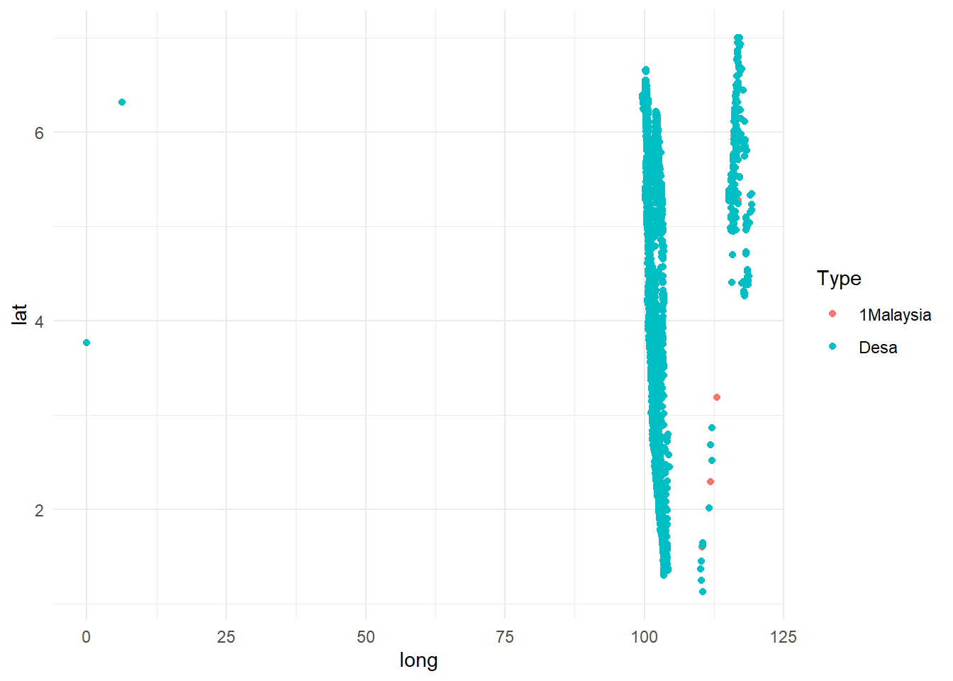

We have 2 isolated points from Klinik Desa data. We will drop these 2 points as well.

all_clinic2 <- all_clinic %>% filter(long > 25)

Plotting the map

There are 2 ways to plot our data to Malaysia map, that we going to cover in this post.

1) map from `ggplot2`

First, we need to get the map.

global <- map_data("world") #get map

Once, we retrieved the map, we need to filter the region to Malaysia. The rest of the codes are ggplot2 function as we know it.

ggplot() + 
  geom_polygon(data = global %>% filter(region == "Malaysia"), aes(x=long, y = lat, group = group), 
               fill = "gray85") + 
  coord_fixed(1.3) +
  geom_point(data = all_clinic2, aes(x = long, y = lat, group = Type, color = Type, shape = Type)) +
  theme_void() + 
  xlab("Longitude") +
  ylab("Latitude") +
  labs(title = "Klinik 1Malaysia dan Klinik Desa di Malaysia", 
       subtitle = "(Data dikemaskini: Klinik 1Malaysia - 16 Mac 2021, Klinik Desa - 9 Mac 2021)",
       caption = expression(paste(italic("Sumber data: https://www.data.gov.my/data/ms_MY/group/pemetaan"))), 
       color = "Jenis klinik:", 
       shape = "Jenis klinik:") +
  theme(plot.title = element_text(hjust = 0.5), 
        plot.subtitle = element_text(hjust = 0.5), 
        legend.position = "bottom")

2) map from `rworldmap`

The flow is similar, we need to get the map first. Then, restrict the map to Malaysia region.

world <- getMap(resolution = "low") #get map
msia <- world[world@data$ADMIN == "Malaysia", ]

The rest of the codes are similar to the first approach. But, we going to change the theme a bit.

ggplot() +
  geom_polygon(data = msia, aes(x = long, y = lat, group = group), fill = NA, colour = "black") +
  geom_point(data = all_clinic2, aes(x = long, y = lat, group = Type, color = Type, shape = Type)) +
  coord_quickmap() + 
  theme_minimal() + 
  xlab("Longitude") +
  ylab("Latitude") +
  labs(title = "Klinik 1Malaysia dan Klinik Desa di Malaysia", 
       subtitle = "(Data dikemaskini: Klinik 1Malaysia - 16 Mac 2021, Klinik Desa - 9 Mac 2021)",
       caption = expression(paste(italic("Sumber data: https://www.data.gov.my/data/ms_MY/group/pemetaan"))), 
       color = "Jenis klinik:", 
       shape = "Jenis klinik:") +
  theme(plot.title = element_text(hjust = 0.5), 
        plot.subtitle = element_text(hjust = 0.5), 
        legend.position = "bottom")

Conclusion

The coordinates that we have are not as accurate as it should, or maybe there is something wrong that I miss along the way. As we can see, we have clinics on the ocean. As far as I know, we Malaysian are not that advanced yet. Also, noticed that we severely lacking clinics in Sarawak, given that our data is correct.

map spatial

Tengku Muhammad Hanis

Lead academic trainer

My research interests include medical statistics and machine learning application.