Data exploration in R

These are some of the packages that I find useful for data exploration. Basically, this post serves more as my note for future reference. I will list out packages (and some awesome functions from that particular package) rather than specific functions. Further, base R and tidyverse packages will not be included specifically in this list.

Load supporting packages

library(tidyverse)

The data we are going to use is from dlookr package:

glimpse(heartfailure)

## Rows: 299
## Columns: 13
## $ age               <int> 75, 55, 65, 50, 65, 90, 75, 60, 65, 80, 75, 62, 45, ~
## $ anaemia           <fct> No, No, No, Yes, Yes, Yes, Yes, Yes, No, Yes, Yes, N~
## $ cpk_enzyme        <dbl> 582, 7861, 146, 111, 160, 47, 246, 315, 157, 123, 81~
## $ diabetes          <fct> No, No, No, No, Yes, No, No, Yes, No, No, No, No, No~
## $ ejection_fraction <dbl> 20, 38, 20, 20, 20, 40, 15, 60, 65, 35, 38, 25, 30, ~
## $ hblood_pressure   <fct> Yes, No, No, No, No, Yes, No, No, No, Yes, Yes, Yes,~
## $ platelets         <dbl> 265000, 263358, 162000, 210000, 327000, 204000, 1270~
## $ creatinine        <dbl> 1.90, 1.10, 1.30, 1.90, 2.70, 2.10, 1.20, 1.10, 1.50~
## $ sodium            <dbl> 130, 136, 129, 137, 116, 132, 137, 131, 138, 133, 13~
## $ sex               <fct> Male, Male, Male, Male, Female, Male, Male, Male, Fe~
## $ smoking           <fct> No, No, Yes, No, No, Yes, No, Yes, No, Yes, Yes, Yes~
## $ time              <int> 4, 6, 7, 7, 8, 8, 10, 10, 10, 10, 10, 10, 11, 11, 12~
## $ death_event       <fct> Yes, Yes, Yes, Yes, Yes, Yes, Yes, Yes, Yes, Yes, Ye~

We will create a few NAs in our data.

set.seed(2021)
heartfailure[sample(seq(nrow(heartfailure)), 20), "age"] <- NA
heartfailure[sample(seq(nrow(heartfailure)), 10), "sex"] <- NA

1) dataMaid

library(dataMaid)

One of the very useful function in dataMaid is makeDataReport() which give report on the data. By default it will give a pdf output, but other output options such as word and html are also available.

makeDataReport(heartfailure, replace = T)

This is the output example in pdf.

2) DataExplorer

library(DataExplorer)

General visualization:

heartfailure %>% plot_intro()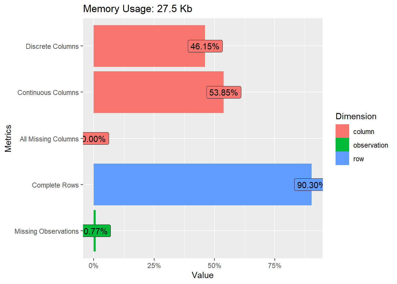

Since we have missing data, we can further visualize it:

heartfailure %>% plot_missing()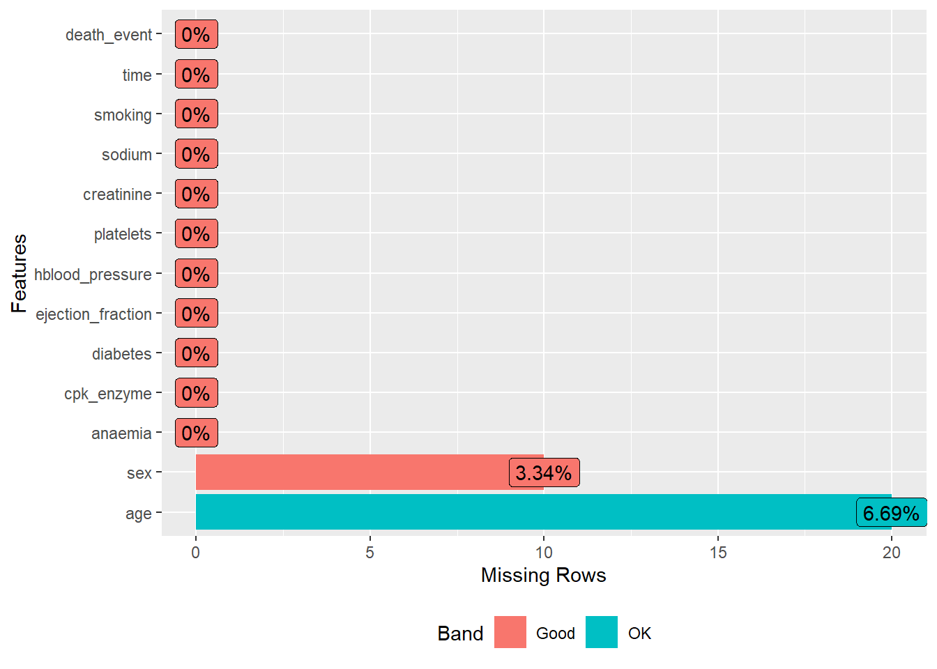

heartfailure %>% profile_missing()

##              feature num_missing pct_missing
## 1                age          20  0.06688963
## 2            anaemia           0  0.00000000
## 3         cpk_enzyme           0  0.00000000
## 4           diabetes           0  0.00000000
## 5  ejection_fraction           0  0.00000000
## 6    hblood_pressure           0  0.00000000
## 7          platelets           0  0.00000000
## 8         creatinine           0  0.00000000
## 9             sodium           0  0.00000000
## 10               sex          10  0.03344482
## 11           smoking           0  0.00000000
## 12              time           0  0.00000000
## 13       death_event           0  0.00000000

We can also do a correlation plot

heartfailure %>% 
  select_if(is.numeric) %>% 
  drop_na() %>% 
  plot_correlation()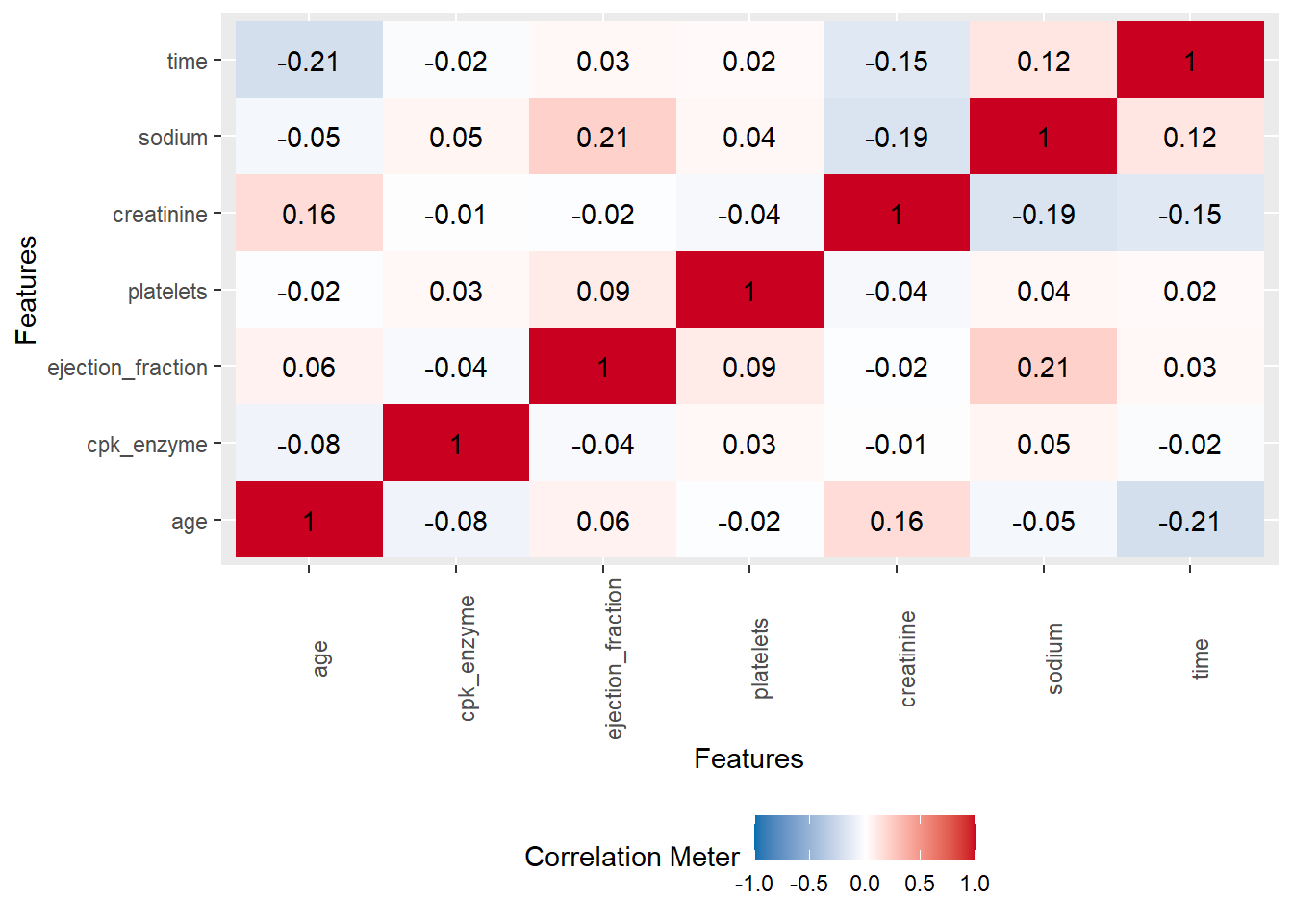

However, I do think correlation plot from corrplot packages gives a better and clean plot. Here is a plot from corrplot.

library(corrplot)

heartfailure %>% 
  select_if(is.numeric) %>% 
  drop_na() %>% 
  cor() %>% 
  corrplot(type = "upper")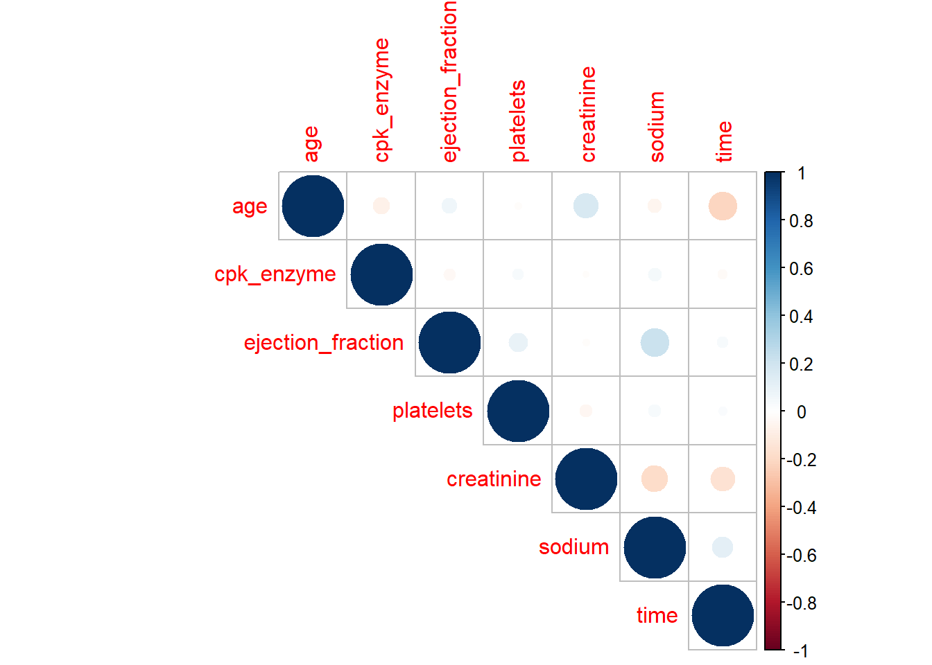

Finally, we can get an overall html report from DataExplorer package using the function create_report().

3) dlookr

library(dlookr)

We can assess normality of the data using this package. The code below will plot normality for all numeric variable.

heartfailure %>% 
  plot_normality()

However, for the sake of the simplicity in this post, we will run only for one variable.

heartfailure %>% 
  plot_normality(age)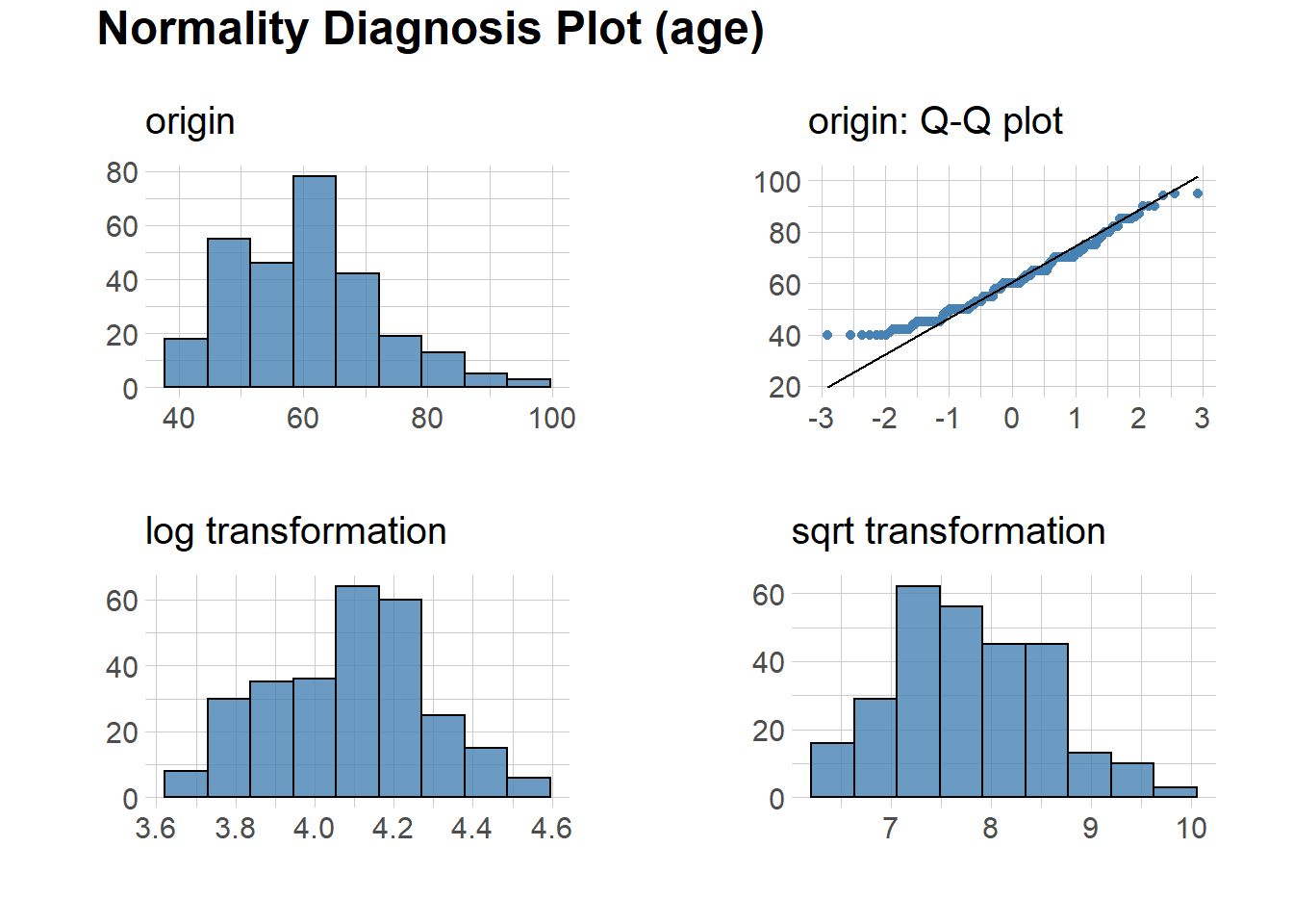

We can also get a correlation matrix plot from this package, and no need to remove the NAs and filter the numeric variable before running the function.

heartfailure %>% 
  plot_correlate()

Lastly, from dlookr we can get the overall report of the data exploration in pdf (and other formats as well). This report is quite comprehensive, have a look.

heartfailure %>% 
  eda_paged_report(target = "death_event")

4) skimr

skimr package, especially skim() function did not display correctly when using the blogdown. Hence, I included the screenshot of the result that we will typically see in the R console.

library(skimr)
skim(heartfailure) 

So, from skimr we can get an overview that includes the histogram for numerical data as well.

5) outliertree

This package identify outlier using a decision tree. I will not go in detail about the approach, but for those who want to read further.

library(outliertree)
outlier.tree(heartfailure)

## Reporting top 2 outliers [out of 2 found]
## 
## row [251] - suspicious column: [creatinine] - suspicious value: [0.50]
##  distribution: 96.000% >= 0.70 - [mean: 1.35] - [sd: 1.22] - [norm. obs: 24]
##  given:
##      [cpk_enzyme] > [1610.00] (value: 2522.00)
## 
## 
## row [32] - suspicious column: [cpk_enzyme] - suspicious value: [23.00]
##  distribution: 98.958% >= 47.00 - [mean: 677.01] - [sd: 1321.86] - [norm. obs: 95]
##  given:
##      [death_event] = [Yes]

## Outlier Tree model
##  Numeric variables: 7
##  Categorical variables: 6
## 
## Consists of 369 clusters, spread across 48 tree branches

We can further explore the detected outliers using histogram and boxplot. Let’s do for variable creatinine.

# histogram
hist(heartfailure$creatinine, breaks = 50, col = "navy",
     xlab = "Creatinine", 
     main = "Creatinine level")

# boxplot
boxplot(heartfailure$creatinine)

Probably in the future I will delve into more detail about outlier detection and any awesome packages in R related to it. If I ever written any post about it, I will link it here.