Variable selection for imputation model in {mice}
Some note
I have written a short post about missing data and multiple imputation in mice package previously. This post will add to that previous post.
Imputation model
Imputation model is the model that we use for our imputation approach. There is another term which is complete-data model. This is a model that we want to fit after we impute the missing values (i.e; the complete-data model is the final model).
Generally, we need to include as many relevant variables into the imputation model. However, this general advise may not be very efficient as we may have multicollinearity and computational issue if we include too many predictors. As a rule of thumb, the number of included variables should be no more than 15-20. van Buuren et al. (2011) mentioned that increased in explained variance in linear regression is negligible after 15 variables are included.
There are 4 steps suggested by van Buuren et al. (1999) for variable selection in the case of big data:
Include all variables that appear in the complete-data model (final model)
- This may include the interaction terms as well (passive imputation can be used to specify the interaction terms in
micepackage)
- This may include the interaction terms as well (passive imputation can be used to specify the interaction terms in
Include variable that have influence on the occurrence of the missing data
- This can be assessed by a correlation matrix between NAs variables and non-NAs variables
Include variable that explain a considerable amount of variance
- This can be crudely assessed by a correlation matrix between NAs variables and non-NAs variables
Remove variable that have too many missing values within the subgroup of incomplete cases
- This can be assessed by a proportion of usable cases (PUC) - how many cases with missing data in a certain variable have an observed values on the predictor variables
All these steps should be done on the key variables only. There is another more efficient yet laborious approach suggested by Oudshoorn et al. (1999), which take into account important predictor of predictors. We are going to focus on the four steps above, and not cover the latter suggested approach in this post.
R codes
These are the required packages.
library(mice)
library(corrplot)
Our data.
summary(airquality)## Ozone Solar.R Wind Temp
## Min. : 1.00 Min. : 7.0 Min. : 1.700 Min. :56.00
## 1st Qu.: 18.00 1st Qu.:115.8 1st Qu.: 7.400 1st Qu.:72.00
## Median : 31.50 Median :205.0 Median : 9.700 Median :79.00
## Mean : 42.13 Mean :185.9 Mean : 9.958 Mean :77.88
## 3rd Qu.: 63.25 3rd Qu.:258.8 3rd Qu.:11.500 3rd Qu.:85.00
## Max. :168.00 Max. :334.0 Max. :20.700 Max. :97.00
## NA's :37 NA's :7
## Month Day
## Min. :5.000 Min. : 1.0
## 1st Qu.:6.000 1st Qu.: 8.0
## Median :7.000 Median :16.0
## Mean :6.993 Mean :15.8
## 3rd Qu.:8.000 3rd Qu.:23.0
## Max. :9.000 Max. :31.0
## We have 2 variables; Ozone and Solar.R with missing values or NAs. We can further explore the pattern of missing variable.
md.pattern(airquality)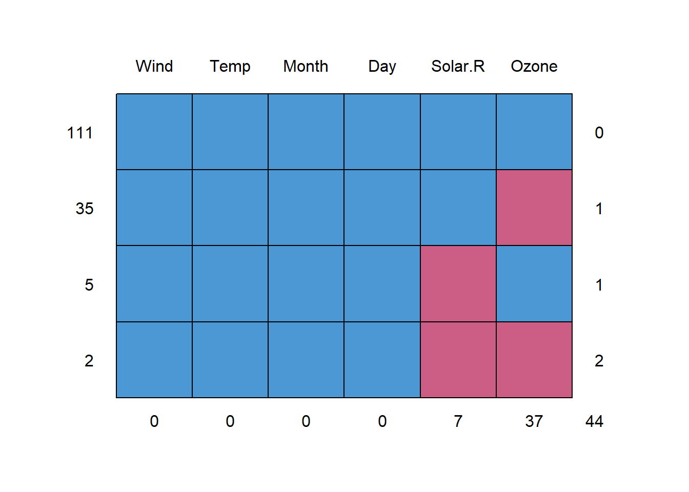
##     Wind Temp Month Day Solar.R Ozone
## 111    1    1     1   1       1     1  0
## 35     1    1     1   1       1     0  1
## 5      1    1     1   1       0     1  1
## 2      1    1     1   1       0     0  2
##        0    0     0   0       7    37 44
There are 2 rows with NAs in Ozone and Solar.R, 35 rows with NAs only in Ozone, and 5 rows with NAs only in Solar.R. Next, we can check the correlation.
cor(airquality, use = "pairwise.complete.obs") |>
  corrplot(method = "number", type = "upper")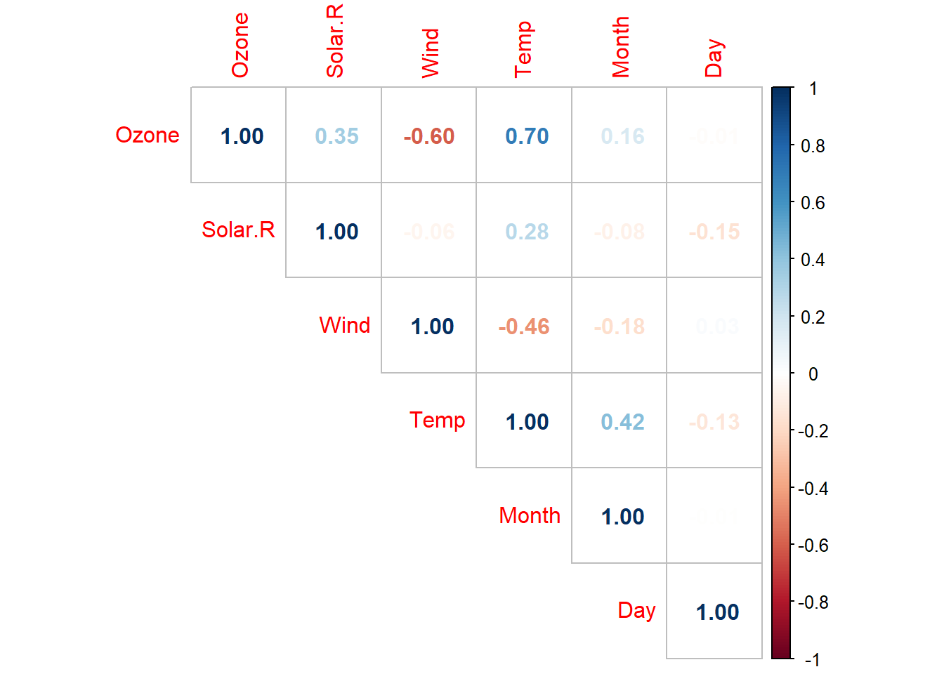
The correlations of Ozone-Temp and Ozone-Wind are the highest. Now, let’s do a correlation between the NAs variable and non-NAs variable.
cor(y = airquality, x = !is.na(airquality), use = "pairwise.complete.obs") |>
  round(digits = 2)
## Ozone Solar.R Wind Temp Month Day
## Ozone NA -0.02 -0.05 0.00 0.26 -0.05
## Solar.R 0 NA 0.06 0.11 0.11 0.17
## Wind NA NA NA NA NA NA
## Temp NA NA NA NA NA NA
## Month NA NA NA NA NA NA
## Day NA NA NA NA NA NAWe can ignore the warnings and the NAs as only Ozone and Solar.R have a missing values. So, the highest correlation is 0.26 between Month-Ozone - correlation between Month values with Ozone-related NAs and Month values with non-Ozone-related NAs. The column variable in the correlation matrix is the indicators of NAs and the row variables is the variable with observed values.
Lastly we can calculate ‘manually’ the PUC (proportion of usable cases). md.pairs() here calculate the number of observation per variable pair.
var_pair <- md.pairs(airquality)
round(var_pair$mr / (var_pair$mr + var_pair$mm), digits = 3)
## Ozone Solar.R Wind Temp Month Day
## Ozone 0.000 0.946 1 1 1 1
## Solar.R 0.714 0.000 1 1 1 1
## Wind NaN NaN NaN NaN NaN NaN
## Temp NaN NaN NaN NaN NaN NaN
## Month NaN NaN NaN NaN NaN NaN
## Day NaN NaN NaN NaN NaN NaNLow value of PUC indicate there is a little information on the predictor to impute the target NAs variable. NaN is shown as the variables have no missing values. The row variable are the target variables to be imputed, and the column variables are the predictors in imputation model. We can see that to impute Solar.R (on the row) Ozone has a little less information (0.714) compare to Wind, Temp, and Day. The diagonal elements will always be 0 or NaN. So, from here we can drop predictors with say, 0 PUC as they contain no information to help impute the target NAs variable.
Actually, we have a nice function from mice that can do what we ‘manually’ did just now.
quickpred(airquality)## Ozone Solar.R Wind Temp Month Day
## Ozone 0 1 1 1 1 0
## Solar.R 1 0 0 1 1 1
## Wind 0 0 0 0 0 0
## Temp 0 0 0 0 0 0
## Month 0 0 0 0 0 0
## Day 0 0 0 0 0 0Again, the column variables are the predictors, and the row variables are the target NAs variables. The above matrix is known as predictor matrix, which going to be used in the imputation model. 1 denote a variable included as predictors and 0 vice versa. The two main arguments in quickpred() are:
mincor - if any of the absolute values in the two correlation matrix that we did earlier above 0.1 (default), the predictors will be included in the predictor matrix
minpuc - the default values for PUC is 0, so the predictors are retained even if they have no information to help imputation model
Notice that, variable Day is excluded from the predictors of Ozone. The correlation values are 0 and -0.05 from the first and second correlation matrices, respectively which do not exceed the default setting of 0.1. That’s why, variable Day is excluded. Also, we can observe a similar situation for variable Wind , which is excluded from the predictors of Solar.R (the correlation coefficients are -0.60 and 0.06). The negative (-) sign does not matter as we actually evaluate the absolute values.
Intuitively, we can change these two arguments as we see fit to do a variable selection for imputation model. Once we finalise our variable selection, we can do the multiple imputation using mice().
# Finalised variable selection
var_sel <- quickpred(airquality)
var_sel## Ozone Solar.R Wind Temp Month Day
## Ozone 0 1 1 1 1 0
## Solar.R 1 0 0 1 1 1
## Wind 0 0 0 0 0 0
## Temp 0 0 0 0 0 0
## Month 0 0 0 0 0 0
## Day 0 0 0 0 0 0# Impute
imp <- mice(airquality, m = 5, predictorMatrix = var_sel, printFlag = F)
imp## Class: mids
## Number of multiple imputations: 5
## Imputation methods:
## Ozone Solar.R Wind Temp Month Day
## "pmm" "pmm" "" "" "" ""
## PredictorMatrix:
##         Ozone Solar.R Wind Temp Month Day
## Ozone       0       1    1    1     1   0
## Solar.R     1       0    0    1     1   1
## Wind        0       0    0    0     0   0
## Temp        0       0    0    0     0   0
## Month       0       0    0    0     0   0
## Day 0 0 0 0 0 0Notice that mice() uses the predictor matrix that we provide.
References:
https://www.jstatsoft.org/article/view/v045i03 - paper written by Staf van Buuren (a bit outdated in terms of codes, but runnable)
https://stefvanbuuren.name/fimd/ - online book written by Stef van Buuren (See chapter 6.3.2 and 9.1.6)
Tengku Muhammad Hanis
Lead academic trainer
My research interests include medical statistics and machine learning application.