A short note on variable selection

Variable selection

Variable or feature selection is one of the important step whether in machine learning or statistical analysis. This post is geared more to the machine learning side. Certain machine learning models such as Support vector machine (SVM) and neural network do not handle irrelevant predictors very well, whereas models such as linear and logistic regression do not handle correlated predictors very well. Thus, careful selection of the variables will help mitigate this issue and further improve the predictive performance.

There are three types of approaches in variable selection:

1. Intrinsic (or built-in feature selection)

An intrinsic feature selection is a feature selection embedded in the algorithm. Some examples include:

1. Tree-and-rule-based model - decision tree, random forest, etc
   
2. Multivariate adaptive regression spline (MARS)
   
3. Regularization method such as least absolute shrinkage and selection operator (LASSO or L1)

Advantages of this type of approach are they are fast and computationally efficient. However, the best variable selected in this approach is model dependent.

2. Filter

In filter approach we determine the variable importance, usually separately though not necessarily. An example of this approach is univariate filter. If the outcome is two categories, we can use t-test to assess the numerical predictors. Variables with a significant p-value or a large t-statistics will be chosen.

This approach is very simple and fast. However, the best subset of variables selected using some filtering criteria such as statistical significance may not reflect the best predictive performance of the model. Additionally, this approach is prone to over-selection of the predictors.

3. Wrapper

There two types of wrapper approaches:

1. Greedy wrapper

Greedy approach or algorithm direct a search path towards the best at times to achieve the best immediate benefit. Due to this reason this approach cannot escape local minima. We can assume in Figure 1 below local minima represents locally best predictors and global minima represents globally best predictors.

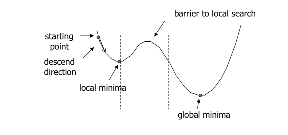
Figure 1: Local minima and global minima

An example of this approach is recursive feature elimination or backward selection. The main weakness of this greedy approach is the selected subset of features identified by this approach may not has the best predictive performance.

2. Non-greedy wrapper

The examples of this approach are simulated annealing and genetic algorithm. Both of these algorithm incorporate a randomness in their approach. Hence, it is classified as non-greedy wrapper. Due to this randomness, it can escape a local minima (see Figure 1 above).

The wrapper type has the best chance to find the globally best predictors. However, this approach is computationally expensive. Not to mention, this approach has a tendency to overfit (some packages like caret use resampling to avoid this issue).

Suggested approach

Kuhn & Johnson (2019) suggested this approach:

1. Start with an intrinsic approach
   

2. Then, do a wrapper approach:

   • If a linear intrinsic approach has a better performance - proceed to wrapper method with a linear model

   • If non-linear intrinsic approach has a better performance - proceed to wrapper method with a non-linear model
     

3. If several approach select a large number of predictors, it may not feasible to reduce the number of features

References:

• https://bookdown.org/max/FES/classes-of-feature-selection-methodologies.html
  
• http://topepo.github.io/caret/feature-selection-overview.html